Study S04 · generated 2026-10-13T21:12:19+00:00 · 319.8 s
Functional network topology across CSDS phases
Neuron-level co-activity graphs, null-model thresholding and graph-theoretic contrasts.
Question
Does the functional network formed by co-active neurons reorganise during defeat and post-defeat sensory contact relative to baseline, and does topology change as defeats accumulate?
Background & rationale
Network neuroscience treats neurons as nodes and statistical dependencies between their activity as edges (Bullmore & Sporns 2009; Rubinov & Sporns 2010). In miniscope data, co-activation graphs built from pairwise correlations, thresholded against shuffled surrogates, reveal stress effects. Repeated stress increases the modularity and degree assortativity of dorsal CA1 networks before coding deficits appear (Transl Psychiatry 2022). Chronic stress also increases between-module cortical connectivity in mesoscale calcium imaging, reversible by ketamine (Neuropsychopharmacology 2022). At the systems level, resilience and susceptibility to CSDS map onto distinct functional connectivity patterns (Mol Psychiatry 2025; Hultman et al. 2018). CaGraph (Porubsky et al.) formalises this approach for calcium imaging.
Methodology
Nodes and edges. Each tracked neuron is a node. For each session, the edge weight between neurons i and j is the Pearson correlation of their inferred spike-probability time series at the native frame rate (150 ms bins, ≈2,000 frames per BL/SD/SS session).
Two complementary thresholds. 1. Statistical graph. Each neuron was circularly shifted independently (shift 10–90% of the session; 50 surrogates). This preserves each neuron's rate and autocorrelation and destroys co-activity. Edges exceed the 99th percentile of the pooled surrogate correlation distribution. Its density (fraction of significant pairs) measures how much genuine co-activity exists. 2. Proportional graph. The strongest 10% of positive correlations. Fixing density removes the trivial dependence of topology on edge count (van Wijk et al. 2010), so this graph is used for all topological measures.
Graph measures (binary, undirected). Clustering coefficient; global efficiency (mean inverse shortest path); characteristic path length (largest component); Louvain modularity Q (resolution 1; Blondel et al. 2008); Q in excess of Q from 3 circular-shift surrogate graphs at the same density; degree assortativity; and small-world σ = (C/C_rand)/(L/L_rand) with Erdős–Rényi approximations (Humphries & Gurney 2008).
Statistics. Primary contrasts use days 1–9, day 7 excluded, restricted to days on which the animal has all of BL, SD and SS: per-animal means compared with a Friedman test and exact Wilcoxon signed-rank tests (SD vs BL, SS vs BL, SS vs SD). Session-level OLS with animal × day block fixed effects gives within-day effect estimates; adding the session mean event rate as a covariate shows how much of each effect firing rate accounts for. These session-level p-values are descriptive (sessions of one animal are not independent). Day trends within SD and BL are tested on per-animal slopes (exact Wilcoxon). P-values were FDR-corrected across all metrics × contrasts, and separately across day trends.
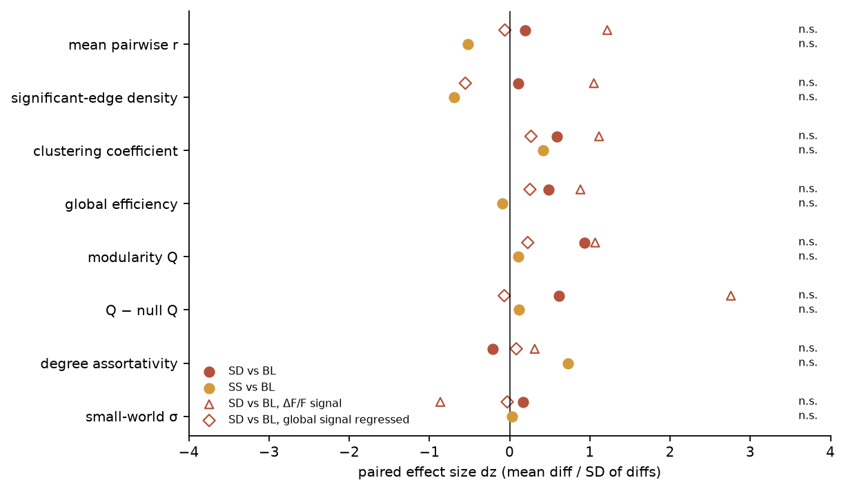
Sensitivity analyses. (i) ΔF/F instead of spike probability; (ii) global signal regression: each neuron's activity is residualised on the population mean before correlation, which removes shared population-wide fluctuations (Murphy & Fox 2017); (iii) SIT CD-1 vs empty phase. Session assignment for the two short recordings is the lab's (6597 lacks SS on day 9; 6669 lacks SIT), so those animals stay in the primary set.
Parameters
| Parameter | Value |
|---|---|
proportional_density | 0.1 |
null_shuffles | 50 |
null_quantile | 0.99 |
louvain_resolution | 1.0 |
seed | 0 |
signal | CASCADE spike probability |
Highlights
null
modularity Q (SD vs BL)
+0.0225
Median paired change; 5/6 animals increased; p = 0.062, q = 0.750; Friedman p = 0.311.
null
clustering coefficient (SD vs BL)
+0.0117
Median paired change; 4/6 animals increased; p = 0.219, q = 0.750; Friedman p = 0.846.
null
Q − null Q (SD vs BL)
+0.0352
Median paired change; 4/6 animals increased; p = 0.219, q = 0.750; Friedman p = 0.607.
null
Robust to sensitivity analyses
0 metric(s)
No SD vs BL effect was both nominally significant and direction-consistent across sensitivity analyses.
Results
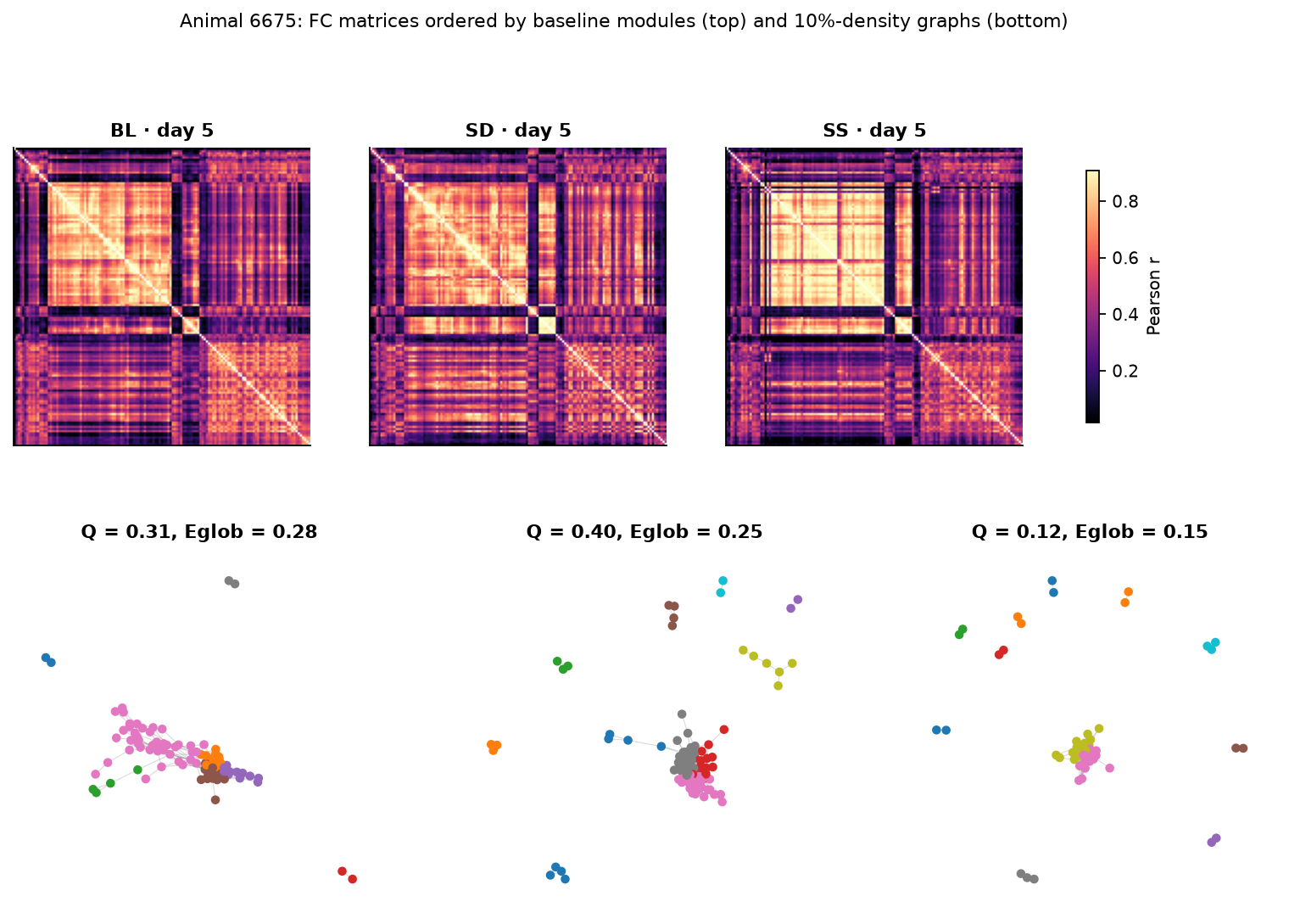
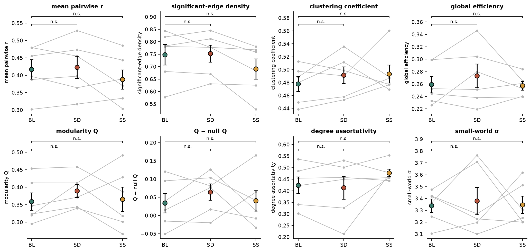
Co-activity. The statistical graphs show how much co-activity exceeds the surrogate null. Significant-edge density averaged BL 0.748, SD 0.752, SS 0.691 (Friedman p = 0.042), and mean pairwise correlation averaged BL 0.417, SD 0.423, SS 0.388 (Friedman p = 0.513). Pairwise correlations are high overall, which indicates a strong shared (population-wide) component in the signal.
Topology at fixed density. The SD vs BL contrasts with the smallest p-values were modularity Q: median Δ = +0.0225 (5/6 animals up, p = 0.062, q = 0.750); clustering coefficient: median Δ = +0.0117 (4/6 animals up, p = 0.219, q = 0.750); Q − null Q: median Δ = +0.0352 (4/6 animals up, p = 0.219, q = 0.750). 0 of 24 metric × contrast tests survived FDR correction. All values are in Table 1 and Figures 2–3.
Confounds and robustness. Table 2 repeats the fixed-effect models with the session firing rate as a covariate; condition terms that shrink markedly are rate-driven. Direction-consistent SD vs BL effects across signal (ΔF/F) and global-signal-regression analyses: none (Table 3, Figure 3).
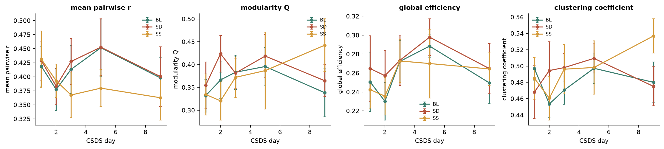
Across defeat days. 0 of 16 day trends survived FDR correction (Table 4, Figure 4).
Figures
Tables
Table 1. Network topology: condition contrasts (days 1–9 without day 7)
| metric | contrast | n | median_diff | dz | n_increase | p | q_fdr | friedman_chi2 | friedman_p |
|---|---|---|---|---|---|---|---|---|---|
| mean_r | SD vs BL | 6 | 0.0124 | 0.196 | 4 | 0.844 | 0.964 | 1.33 | 0.513 |
| mean_r | SS vs BL | 6 | -0.0095 | -0.524 | 2 | 0.312 | 0.938 | 1.33 | 0.513 |
| mean_r | SS vs SD | 6 | -0.0365 | -0.701 | 2 | 0.156 | 0.75 | 1.33 | 0.513 |
| sig_density | SD vs BL | 6 | 0.0112 | 0.108 | 3 | 0.844 | 0.964 | 6.33 | 0.0421 |
| sig_density | SS vs BL | 6 | -0.0315 | -0.691 | 1 | 0.219 | 0.75 | 6.33 | 0.0421 |
| sig_density | SS vs SD | 6 | -0.0587 | -1.19 | 0 | 0.0312 | 0.75 | 6.33 | 0.0421 |
| prop_clustering | SD vs BL | 6 | 0.0117 | 0.588 | 4 | 0.219 | 0.75 | 0.333 | 0.846 |
| prop_clustering | SS vs BL | 6 | 0.0187 | 0.416 | 3 | 0.438 | 0.964 | 0.333 | 0.846 |
| prop_clustering | SS vs SD | 6 | 0.000724 | 0.0381 | 3 | 1 | 1 | 0.333 | 0.846 |
| prop_efficiency | SD vs BL | 6 | 0.00184 | 0.487 | 3 | 0.688 | 0.964 | 0 | 1 |
| prop_efficiency | SS vs BL | 6 | 0.000994 | -0.0918 | 3 | 1 | 1 | 0 | 1 |
| prop_efficiency | SS vs SD | 6 | -0.00958 | -0.439 | 3 | 0.562 | 0.964 | 0 | 1 |
| prop_modularity | SD vs BL | 6 | 0.0225 | 0.929 | 5 | 0.0625 | 0.75 | 2.33 | 0.311 |
| prop_modularity | SS vs BL | 6 | 0.0019 | 0.106 | 3 | 0.688 | 0.964 | 2.33 | 0.311 |
| prop_modularity | SS vs SD | 6 | -0.0548 | -0.324 | 2 | 0.562 | 0.964 | 2.33 | 0.311 |
| prop_modularity_excess | SD vs BL | 6 | 0.0352 | 0.611 | 4 | 0.219 | 0.75 | 1 | 0.607 |
| prop_modularity_excess | SS vs BL | 6 | 0.00868 | 0.117 | 3 | 1 | 1 | 1 | 0.607 |
| prop_modularity_excess | SS vs SD | 6 | -0.0435 | -0.263 | 2 | 0.562 | 0.964 | 1 | 0.607 |
| prop_assortativity | SD vs BL | 6 | -0.00583 | -0.215 | 3 | 0.844 | 0.964 | 1 | 0.607 |
| prop_assortativity | SS vs BL | 6 | 0.0259 | 0.726 | 4 | 0.156 | 0.75 | 1 | 0.607 |
| prop_assortativity | SS vs SD | 6 | 0.0298 | 0.556 | 4 | 0.438 | 0.964 | 1 | 0.607 |
| prop_small_world | SD vs BL | 6 | -0.0282 | 0.164 | 3 | 0.844 | 0.964 | 0.333 | 0.846 |
| prop_small_world | SS vs BL | 6 | -0.0342 | 0.0279 | 2 | 0.844 | 0.964 | 0.333 | 0.846 |
| prop_small_world | SS vs SD | 6 | 0.0551 | -0.0848 | 3 | 0.844 | 0.964 | 0.333 | 0.846 |
Table 2. Session-level models with and without a firing-rate covariate
| metric | term | coef | se | p_session | n_sessions | model |
|---|---|---|---|---|---|---|
| mean_r | SD vs BL | 0.00726 | 0.0168 | 0.668 | 87 | condition + animal |
| mean_r | SS vs BL | -0.0296 | 0.0168 | 0.084 | 87 | condition + animal |
| sig_density | SD vs BL | 0.00368 | 0.0241 | 0.879 | 87 | condition + animal |
| sig_density | SS vs BL | -0.0582 | 0.0241 | 0.0189 | 87 | condition + animal |
| prop_clustering | SD vs BL | 0.013 | 0.0146 | 0.379 | 87 | condition + animal |
| prop_clustering | SS vs BL | 0.0163 | 0.0146 | 0.271 | 87 | condition + animal |
| prop_efficiency | SD vs BL | 0.013 | 0.0128 | 0.313 | 87 | condition + animal |
| prop_efficiency | SS vs BL | -0.000837 | 0.0128 | 0.948 | 87 | condition + animal |
| prop_modularity | SD vs BL | 0.031 | 0.0259 | 0.237 | 87 | condition + animal |
| prop_modularity | SS vs BL | 0.00897 | 0.0259 | 0.731 | 87 | condition + animal |
| prop_modularity_excess | SD vs BL | 0.0291 | 0.0289 | 0.319 | 87 | condition + animal |
| prop_modularity_excess | SS vs BL | 0.00848 | 0.0289 | 0.77 | 87 | condition + animal |
| prop_assortativity | SD vs BL | -0.00767 | 0.0335 | 0.82 | 87 | condition + animal |
| prop_assortativity | SS vs BL | 0.0493 | 0.0335 | 0.147 | 87 | condition + animal |
| prop_small_world | SD vs BL | 0.0333 | 0.112 | 0.767 | 87 | condition + animal |
| prop_small_world | SS vs BL | 0.0175 | 0.112 | 0.876 | 87 | condition + animal |
| mean_r | SD vs BL | 0.0153 | 0.0202 | 0.45 | 87 | + rate covariate |
| mean_r | SS vs BL | -0.0275 | 0.0172 | 0.115 | 87 | + rate covariate |
| sig_density | SD vs BL | 0.0207 | 0.0287 | 0.473 | 87 | + rate covariate |
| sig_density | SS vs BL | -0.0537 | 0.0244 | 0.0318 | 87 | + rate covariate |
| prop_clustering | SD vs BL | -0.000739 | 0.0173 | 0.966 | 87 | + rate covariate |
| prop_clustering | SS vs BL | 0.0127 | 0.0147 | 0.392 | 87 | + rate covariate |
| prop_efficiency | SD vs BL | 0.00591 | 0.0153 | 0.7 | 87 | + rate covariate |
| prop_efficiency | SS vs BL | -0.0027 | 0.013 | 0.836 | 87 | + rate covariate |
| prop_modularity | SD vs BL | -0.00332 | 0.03 | 0.912 | 87 | + rate covariate |
| prop_modularity | SS vs BL | -3.78e-05 | 0.0255 | 0.999 | 87 | + rate covariate |
| prop_modularity_excess | SD vs BL | 0.00852 | 0.0344 | 0.805 | 87 | + rate covariate |
| prop_modularity_excess | SS vs BL | 0.00309 | 0.0293 | 0.916 | 87 | + rate covariate |
| prop_assortativity | SD vs BL | 0.00959 | 0.0401 | 0.812 | 87 | + rate covariate |
| prop_assortativity | SS vs BL | 0.0538 | 0.0341 | 0.12 | 87 | + rate covariate |
| prop_small_world | SD vs BL | -0.015 | 0.134 | 0.911 | 87 | + rate covariate |
| prop_small_world | SS vs BL | 0.00485 | 0.114 | 0.966 | 87 | + rate covariate |
Table 3. Sensitivity analyses (SD vs BL unless stated)
| metric | analysis | contrast | n | median_diff | mean_diff | n_increase | p | dz |
|---|---|---|---|---|---|---|---|---|
| mean_r | ΔF/F signal | SD vs BL | 6 | 0.0314 | 0.0364 | 5 | 0.0625 | 1.22 |
| mean_r | global signal regressed | SD vs BL | 6 | -0.000242 | -0.000733 | 3 | 1 | -0.0597 |
| mean_r | SIT CD1 vs empty | SIT_CD1 vs SIT_NoCD1 | 5 | 0.0509 | 0.0327 | 3 | 0.438 | 0.526 |
| sig_density | ΔF/F signal | SD vs BL | 6 | 0.0419 | 0.0472 | 5 | 0.0625 | 1.05 |
| sig_density | global signal regressed | SD vs BL | 6 | -0.00737 | -0.00754 | 2 | 0.312 | -0.552 |
| sig_density | SIT CD1 vs empty | SIT_CD1 vs SIT_NoCD1 | 5 | 0.116 | 0.125 | 4 | 0.125 | 0.88 |
| prop_clustering | ΔF/F signal | SD vs BL | 6 | 0.0263 | 0.0225 | 5 | 0.0938 | 1.11 |
| prop_clustering | global signal regressed | SD vs BL | 6 | 0.00953 | 0.00655 | 3 | 0.688 | 0.266 |
| prop_clustering | SIT CD1 vs empty | SIT_CD1 vs SIT_NoCD1 | 5 | -0.0151 | -0.0127 | 2 | 1 | -0.146 |
| prop_efficiency | ΔF/F signal | SD vs BL | 6 | 0.0335 | 0.0223 | 5 | 0.0938 | 0.882 |
| prop_efficiency | global signal regressed | SD vs BL | 6 | 0.00437 | 0.00798 | 3 | 0.688 | 0.253 |
| prop_efficiency | SIT CD1 vs empty | SIT_CD1 vs SIT_NoCD1 | 5 | -0.0576 | -0.0274 | 1 | 0.438 | -0.241 |
| prop_modularity | ΔF/F signal | SD vs BL | 6 | 0.0462 | 0.0512 | 5 | 0.0625 | 1.07 |
| prop_modularity | global signal regressed | SD vs BL | 6 | 0.0193 | 0.0116 | 4 | 0.688 | 0.226 |
| prop_modularity | SIT CD1 vs empty | SIT_CD1 vs SIT_NoCD1 | 5 | -0.0392 | -0.00919 | 2 | 0.812 | -0.0633 |
| prop_modularity_excess | ΔF/F signal | SD vs BL | 6 | 0.048 | 0.0519 | 6 | 0.0312 | 2.76 |
| prop_modularity_excess | global signal regressed | SD vs BL | 6 | 0.0206 | -0.00521 | 4 | 1 | -0.0669 |
| prop_modularity_excess | SIT CD1 vs empty | SIT_CD1 vs SIT_NoCD1 | 5 | -0.0138 | -0.000991 | 1 | 0.625 | -0.0059 |
| prop_assortativity | ΔF/F signal | SD vs BL | 6 | 0.0148 | 0.0294 | 4 | 0.562 | 0.312 |
| prop_assortativity | global signal regressed | SD vs BL | 6 | 0.0162 | 0.00568 | 4 | 0.844 | 0.0824 |
| prop_assortativity | SIT CD1 vs empty | SIT_CD1 vs SIT_NoCD1 | 5 | 0.0568 | 0.0476 | 3 | 0.312 | 0.73 |
| prop_small_world | ΔF/F signal | SD vs BL | 6 | -0.196 | -0.199 | 1 | 0.0938 | -0.864 |
| prop_small_world | global signal regressed | SD vs BL | 6 | -0.0766 | -0.0092 | 2 | 0.844 | -0.0299 |
| prop_small_world | SIT CD1 vs empty | SIT_CD1 vs SIT_NoCD1 | 5 | -0.0686 | -0.227 | 2 | 0.625 | -0.327 |
Table 4. Day trends of topology
| metric | condition | slope_per_day | median_animal_slope | n_positive | n_animals | p | n_sessions | q_fdr |
|---|---|---|---|---|---|---|---|---|
| mean_r | SD | -0.000638 | 0.00124 | 4 | 6 | 0.844 | 30 | 1 |
| mean_r | BL | 0.000442 | 0.0037 | 4 | 6 | 0.688 | 30 | 1 |
| sig_density | SD | 0.00388 | 0.00689 | 4 | 6 | 0.562 | 30 | 1 |
| sig_density | BL | 0.0117 | 0.0132 | 5 | 6 | 0.219 | 30 | 1 |
| prop_clustering | SD | -0.000169 | -0.002 | 3 | 6 | 1 | 30 | 1 |
| prop_clustering | BL | 0.000737 | 0.00263 | 4 | 6 | 1 | 30 | 1 |
| prop_efficiency | SD | 0.000996 | 0.00174 | 4 | 6 | 0.844 | 30 | 1 |
| prop_efficiency | BL | 0.00131 | 0.000272 | 4 | 6 | 0.688 | 30 | 1 |
| prop_modularity | SD | -0.00126 | -0.00662 | 1 | 6 | 0.438 | 30 | 1 |
| prop_modularity | BL | -0.000594 | 0.00216 | 3 | 6 | 1 | 30 | 1 |
| prop_modularity_excess | SD | 0.0027 | -0.00478 | 2 | 6 | 0.688 | 30 | 1 |
| prop_modularity_excess | BL | 0.00309 | 0.00139 | 3 | 6 | 0.688 | 30 | 1 |
| prop_assortativity | SD | -0.00198 | -0.0137 | 2 | 6 | 0.844 | 30 | 1 |
| prop_assortativity | BL | 0.000367 | -0.000672 | 3 | 6 | 1 | 30 | 1 |
| prop_small_world | SD | -0.00428 | -0.0185 | 2 | 6 | 0.844 | 30 | 1 |
| prop_small_world | BL | -0.00221 | 0.00173 | 3 | 6 | 1 | 30 | 1 |
Table 5. All session-level network measures
| key | subject | condition | day | mapping | n_neurons | n_frames | mean_rate | mean_r | mean_pos_r | null_thr | sig_density | prop_density | prop_mean_degree | prop_clustering | prop_path_length | prop_efficiency | prop_modularity | prop_n_modules | prop_assortativity | prop_small_world | prop_lcc_fraction | prop_modularity_null | prop_modularity_excess |
|---|---|---|---|---|---|---|---|---|---|---|---|---|---|---|---|---|---|---|---|---|---|---|---|
| 4703_BL_D1 | 4703 | BL | 1 | supported | 105 | 1967 | 1.75 | 0.414 | 0.429 | 0.24 | 0.675 | 0.1 | 10.4 | 0.49 | 2.67 | 0.23 | 0.374 | 5 | 0.52 | 3.66 | 0.676 | 0.347 | 0.0267 |
| 4703_SD_D1 | 4703 | SD | 1 | supported | 105 | 2001 | 1.79 | 0.506 | 0.551 | 0.338 | 0.634 | 0.1 | 10.4 | 0.354 | 2.5 | 0.147 | 0.173 | 6 | 0.45 | 2.81 | 0.486 | 0.525 | -0.353 |
| 4703_SS_D1 | 4703 | SS | 1 | supported | 105 | 2000 | 1.9 | 0.438 | 0.531 | 0.262 | 0.637 | 0.1 | 10.4 | 0.48 | 3.13 | 0.223 | 0.412 | 5 | 0.501 | 3.05 | 0.686 | 0.375 | 0.0376 |
| 4703_BL_D2 | 4703 | BL | 2 | supported | 105 | 2000 | 1.85 | 0.427 | 0.498 | 0.28 | 0.634 | 0.1 | 10.4 | 0.448 | 3.12 | 0.223 | 0.375 | 4 | 0.528 | 2.85 | 0.695 | 0.418 | -0.0434 |
| 4703_SD_D2 | 4703 | SD | 2 | supported | 105 | 2001 | 2.09 | 0.476 | 0.516 | 0.29 | 0.653 | 0.1 | 10.4 | 0.441 | 3.15 | 0.206 | 0.371 | 6 | 0.703 | 2.78 | 0.657 | 0.381 | -0.00996 |
| 4703_SS_D2 | 4703 | SS | 2 | supported | 105 | 2000 | 1.86 | 0.47 | 0.51 | 0.3 | 0.674 | 0.1 | 10.4 | 0.421 | 2.99 | 0.196 | 0.353 | 4 | 0.562 | 2.79 | 0.629 | 0.413 | -0.0601 |
| 4703_BL_D3 | 4703 | BL | 3 | supported | 105 | 2000 | 1.73 | 0.465 | 0.485 | 0.201 | 0.817 | 0.1 | 10.4 | 0.398 | 3.15 | 0.239 | 0.281 | 6 | 0.318 | 2.51 | 0.724 | 0.332 | -0.0503 |
| 4703_SD_D3 | 4703 | SD | 3 | supported | 105 | 2000 | 1.85 | 0.512 | 0.525 | 0.266 | 0.761 | 0.1 | 10.4 | 0.534 | 3.07 | 0.262 | 0.443 | 7 | 0.376 | 3.46 | 0.762 | 0.399 | 0.0439 |
| 4703_SS_D3 | 4703 | SS | 3 | supported | 105 | 2001 | 1.77 | 0.517 | 0.522 | 0.157 | 0.893 | 0.1 | 10.4 | 0.463 | 2.87 | 0.247 | 0.354 | 6 | 0.391 | 3.21 | 0.724 | 0.334 | 0.02 |
| 4703_BL_D5 | 4703 | BL | 5 | supported | 105 | 2000 | 1.41 | 0.685 | 0.685 | 0.251 | 0.962 | 0.1 | 10.4 | 0.443 | 2.38 | 0.246 | 0.344 | 8 | 0.266 | 3.7 | 0.686 | 0.404 | -0.0593 |
| 4703_SD_D5 | 4703 | SD | 5 | supported | 105 | 2000 | 1.57 | 0.673 | 0.673 | 0.206 | 0.976 | 0.1 | 10.4 | 0.455 | 2.95 | 0.245 | 0.361 | 9 | 0.512 | 3.06 | 0.724 | 0.338 | 0.0229 |
| 4703_SS_D5 | 4703 | SS | 5 | supported | 105 | 2001 | 1.49 | 0.513 | 0.513 | 0.279 | 0.812 | 0.1 | 10.4 | 0.572 | 3.12 | 0.292 | 0.516 | 5 | 0.395 | 3.64 | 0.829 | 0.357 | 0.16 |
Limitations
- Pearson correlations of calcium-derived signals reflect shared input and common modulation as well as synaptic coupling. Edges are functional, not anatomical.
- Correlations rise with firing rate (de la Rocha et al. 2007). The rate-covariate model addresses this partially.
- Mean pairwise correlations are high (≈0.4–0.7), consistent with a strong shared component (global co-fluctuation, residual neuropil or motion). Proportional graphs keep the strongest edges, which partly mitigates this. The global-signal-regressed sensitivity analysis tests whether effects survive removing it. Global signal regression can itself introduce negative correlations, so neither version is definitive.
- The proportional threshold (10%) is a choice. Effects consistent across the statistical and proportional graphs are more trustworthy.
- n = 6 animals, no unstressed control group: condition effects are within-animal contrasts of contexts, not stress-vs-control comparisons.
- BL, SD and SS are always recorded in that order within a day, so condition contrasts are confounded with position in the recording.
- Small-world σ uses Erdős–Rényi approximations (C_rand = k/(n−1), L_rand = ln n / ln k), with C over all nodes and L over the largest component. It is a relative index, not an absolute small-world test.
References
- Bullmore E. & Sporns O. (2009) Complex brain networks: graph theoretical analysis of structural and functional systems. Nat Rev Neurosci 10:186–198.
- Murphy K. & Fox M.D. (2017) Towards a consensus regarding global signal regression for resting state functional connectivity MRI. NeuroImage 154:169–173.
- Rubinov M. & Sporns O. (2010) Complex network measures of brain connectivity: uses and interpretations. NeuroImage 52:1059–1069.
- Repeated stress exposure leads to structural synaptic instability prior to disorganization of hippocampal coding (2022) Transl Psychiatry. doi:10.1038/s41398-022-02107-5
- Selective effects of acute and chronic stress on cortical functional connectivity and reversal with ketamine (2022) Neuropsychopharmacology. doi:10.1038/s41386-022-01506-y
- Resting-state fMRI reveals altered functional connectivity associated with resilience and susceptibility to CSDS (2025) Mol Psychiatry. doi:10.1038/s41380-025-02897-2
- Hultman R. et al. (2018) Brain-wide electrical spatiotemporal dynamics encode depression vulnerability. Cell 173:166–180.
- Blondel V.D. et al. (2008) Fast unfolding of communities in large networks. J Stat Mech P10008.
- van Wijk B.C.M., Stam C.J. & Daffertshofer A. (2010) Comparing brain networks of different size and connectivity density using graph theory. PLoS One 5:e13701.
- Humphries M.D. & Gurney K. (2008) Network 'small-world-ness': a quantitative method for determining canonical network equivalence. PLoS One 3:e0002051.
- Porubsky V. et al. CaGraph: graph theory analysis of calcium imaging data. github.com/vporubsky/CaGraph